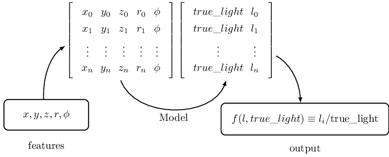
Illustration of functional map

This is a diagram I used to explain the functional model made using Machine Learning library to understand positional characterstics of an arbitrary function.

\tikzset{
  state/.style={
    rectangle, rounded corners, draw=black, thick,
    minimum height=2em, minimum width=8em, inner sep=10pt,
    text centered
  }
}

\begin{tikzpicture}[>=latex, line width=0.75pt]
  \begin{scope}
    \node[state] (modelo1) {$x,y,z,r,\phi$};
    \node[below of=modelo1] {features};
    \node (m1) [above right of=modelo1, node distance=3.5cm,
      matrix of math nodes, left delimiter=[,right delimiter={]}]
      {
          x_0 &  y_0 &  z_0 & r_0 & \phi\\
          x_1 &  y_1 &  z_1 & r_1 & \phi\\
          \vdots &  \vdots &  \vdots & \vdots & \vdots \\
          x_n &  y_n &  z_n & r_n & \phi\\
      };
    \node (m2) [right of=m1, node distance=3.5cm,
      matrix of math nodes, left delimiter=[,right delimiter={]}]
      { 
          true\_light &  l_0 \\
          true\_light &  l_1 \\
          \vdots & \vdots \\
          true\_light &  l_n \\
      };
    \node (modelo2) [below right of=m2, state, node distance=3.7cm]
      (modelo2) {$f(l,true\_light) \equiv l_i/\text{true\_light}$};
    \node[below of=modelo2] {output};
    \path[->, shorten >=1em] (modelo1) edge[bend left=30] (m1.west);
    \path[->] (m1.south) edge[bend right=70]
      node [midway, below] {Model} (m2.south);
    \path[<-, shorten >=1em] (modelo2) edge[bend right=30] (m2);
  \end{scope}
\end{tikzpicture}