Basic Neural Network with multiple nodes

2024-07-28 · Prakash

In the previous two posts we have already seen how to construct a single neuron neural network with or without hidden layer. If we want to input multidimensional input and get multidimensional output from the netwro then we have to add more nodes in each layers so that each node in the layer can process independent multidimensional input. For this purpose in this post we will construct a network with a single output layer but with multiple nodes in input layer. This is useful for example if we want to train our network to learn the scalar (one number) function of \(N\) dimensional vector.

Setup

Similar to last post, where we made a basic neural network with just one neuron and just one hidden layer, we will build multiple neuron network but with a single output.

    %% {init {'theme':'dark'}}%%
    graph LR;
        x_1 --> a1((a_1))-->|W_11| b1((b_1)) --> y1((y_1))
        x_2 --> a2((a_2)) -->|W_21| b1
        x_3 --> a3((a_3)) -->|W_31| b1
        a1 --> |W_12| b2((b_2)) --> y2((y_2))
        a2 --> |W_22| b2
        a3 --> |W_32| b2

The input vector \(x\) passes through the network to the output layer. For the notational consistancy, we can call \(a = x\), where the superscript is index. The output of the network is then

\[ \begin{aligned}y_1 = (W_{11} \cdot a_1 + W_{21} \cdot a_2 + W_{31} \cdot a_3 + b_1)\\ y_2 = (W_{12} \cdot a_1 + W_{22} \cdot a_2 + W_{32} \cdot a_3 + b_2)\end{aligned} \]

If we define our input vector

\[ \begin{aligned}x = \begin{pmatrix}x_1\\ x_2\\ x_3\end{pmatrix} = \begin{pmatrix} a_1\\ a_2\\ a_3 \end{pmatrix}\end{aligned} \]

, the weights in a matrix \(W\)

\[ \begin{aligned}W = \begin{pmatrix}W_{11} & W_{12}\\W_{21} & W_{22}\\ W_{31} & W_{32}\end{pmatrix}\end{aligned} \]

and the output by vector \(y\) as

\[ \begin{aligned}y = \begin{pmatrix}y_1 \\ y_2\end{pmatrix}\end{aligned} \]

We can write the expression for \(y\) simply as

\[ \begin{aligned}y = W^\prime \cdot x + b\end{aligned} \]

This is linear in \(x\) but the input \(x\) is a vector now and the output \(y\) is a vector too.

Lets just extend our basic neural network post for multiple inputs. Because this is a linear network we can only ever expect to learn linear function. So lets take any two linear functions of three variables.

\[ \begin{aligned}y_1 = x_1 + 2x_2 + 3 x_3 + 4\\ y_2 = 3x_1 + 2x_2 + x_3 + 0\\\end{aligned} \]

So we can define our function that we want to model in julia as

Wt = [1 3;
     2 2;
     3 1;
]
bt = [4;
      0
]

f(x) = Wt' * x + bt

Lets again declare the loss function

\[ \begin{aligned}L(y,\hat y) = \left( y - \hat y \right) ^{2}\end{aligned} \]

Where \(y\) is the predicted value and \(\hat y\) is the true value.

In julia this exactly translates as

L(y,ŷ) = sum( (y - ŷ) .^2 )

We can follow the post on back propagation and gradient descent to understand the algorithm. The implementation of the algorithm is exactly same is shown in that post. The (almost) exact copy of that code is here. The only change is that the \(W\) variable is now a matrix and \(b\) is a vector with \(a=x\) being a vector.

function train!(x,y)
    # Feed forward
    a⁰ = x
    a¹ = W' * a⁰ + b

    # Calculate error
    δ¹ = (a¹ - y)
    # Single layer so no backpropagation

    # Updaet weights
    global W -= β .* a⁰ * δ¹'
    global b -= β .* δ¹
    return a¹
end

Training network

Lets first generate some training sample. We want a list of vectors. One I deaa I have for generating training sample is to start with three sets \(x_1 = \lbrace 1, 2, \cdots n\rbrace\), \(x_2 = \lbrace 1, 2, \cdots n\rbrace\) , \(x_3 = \lbrace 1, 2, \cdots n\rbrace\) for each component of vector \(x\) to form the vector just take the cartesian product. For that matter lets define a cartesian product function in julia.

×(x₁,x₂) = [[i;j] for i in x₁ for j in x₂]

We can generate the component set simply as

x1_train,x2_train,x3_train = 1.0:9.0, 1.0:9.0, 1.0:9.0

Finally the training set then is

x_train = x1_train × x2_train × x3_train

For our purpose we can start with any arbitrary weight matrix \(W\) and any arbitrary bias vector \(b\).

W = rand(3,2)
b = vec(rand(2,1))

Lets also set some learning rage \(\beta\)

β = 9e-3

Now we can train the network with our training samples. This again is the exact identical copy of the code in the backpropagation post.

epoch=500
errs = []
for n in 1:epoch
    for (i,(x,y)) in enumerate(zip(x_train,y_train))
        ŷ = train!(x,y)
        error = loss(y,ŷ)
        push!(errs,error)
        print(f"\rEpoch {$n:>2d}: {$i:>02d}/{$(length(x_train)):>02d}   error = {$error:.3e}")
        #sleep(.15)
    end
    println("")
end

Epoch 1: 729/729   error = 1.301e-05
Epoch 2: 729/729   error = 3.603e-07
Epoch 3: 729/729   error = 2.187e-07
Epoch 4: 729/729   error = 1.912e-07
.
.
.
Epoch 496: 729/729   error = 1.010e-28
Epoch 497: 729/729   error = 2.524e-28
Epoch 498: 729/729   error = 8.078e-28
Epoch 499: 729/729   error = 2.524e-28
Epoch 500: 729/729   error = 8.078e-28

We see that the error goes down at the end of each epoch. Telling us that the back propagation works.

We can print the final matrices \(W\) and \(b\) we will see that they are very close to the true values we wanted to start with.

print(W)

3×2 Matrix{Float64}:
1.0000000000001126 2.999999999999939
1.999999999999995  2.000000000000002
2.9999999999999982 1.0000000000000002

print(b)

2-element Vector{Float64}:
 3.9999999999990083
 5.228242039274647e-13

These are indeed the values we wanted \(W\) and \(b\) converge to.

Characterization

I have caught error in each iteration in the array errs which can be used to make few plots. We can reshape the error list such that each row is error progression in each epoch.

ers = reshape(errs,length(x_train),epoch)

Lets plot the final error in each epoch for all the epochs.

le = ers[end,:]

Now we can make plots.

p = plot(xlabel="Epoch",ylabel="MSE",title="Error progression")
plot!(le,label="β=$β")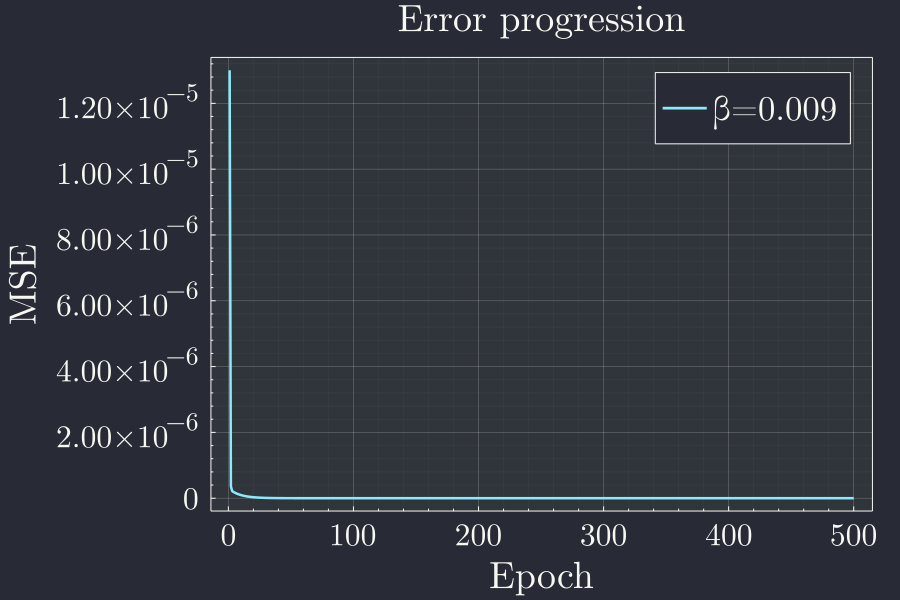

This plot clearly indicates that the error goes very quickly down but there a blog on the left corner. Lets see what's going on there with a log plot.

p = plot(xlabel="Epoch",ylabel="MSE",title="Error progression logy",yscale=:log10)
ylims!(1e-9,1e3)
x = 1:4900
plot!(x,le[x],label="β=$β")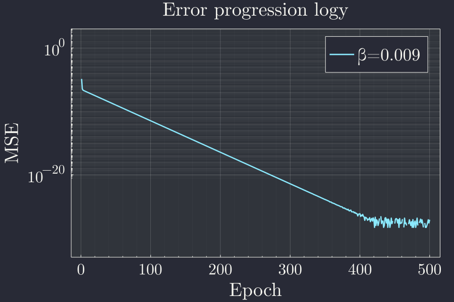

Looks like there is lot of wiggle towards the end but the error stalls there. It rapidly goes down for the first 400 epochs or so. Lets try to catch a single(or a few) wiggle and see what is happening.

p = plot(xlabel="Epoch",ylabel="MSE",title="Error progression logy",yscale=:log10)
ylims!(1e-9,1e3)
x = 250:500
plot!(x,le[x],label="β=$β")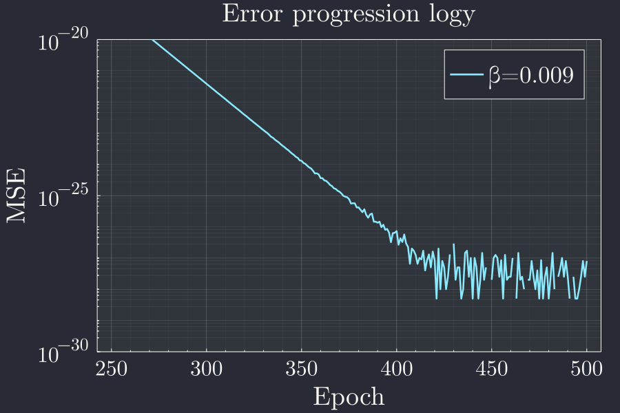

I am not sure what to make of this, but since this is vanishingly small value for error I am not even sure about the precision of the numbers here. Might be worth investigating later.

Conclusion

With almost the same code as for single node in each layer, we are able to simply turn the Weights and biases into matrix and be able to handle the multiple node in each layer case very easily. Its so nice to also learn that the linear learnign works quite well when there is mixing of input variables in the output.

Now that we have built a neural network with single layer, two layers and multiple nodes in each layers, our next big target is to make a network with all these. Apply backpropagation to a multilayered network with multiple node in ecah layer. That shold be the ultimate linear regression neural network. Until then bye. Adios, hasta pronto.