Basic Neural Network with activation function

2024-07-28 · Prakash

As we saw in previous post addition of any number of layers and any number of nodes will only be able to model a linear functions. If we want our network to also be able to learn non linear functions, then we should introduce some non linearlity to the network. One way of adding non linearity is to use so called activation function. The idea is that we pass the output of each layer through a (non linear) function. Our examples so far can be considered to have been using a linear activation function. In particular, they all used identity activation function

Setup

Similar to last post we will build a two neuron and a single hidden layer.

%% {init {'theme':'dark'}} %% flowchart LR; x --> a((a⁰))-->|W¹| b((b¹))-->|W²| c((b²)) --> y

The input \(x\) passes through one hidden layer finally to the output layer. For the notational consistancy, we can call \(a^0 = x\), where the superscript is index. Let us introduce an intermediate variable \(z\), for the first layer it is defined as.

\[ \begin{aligned}z^1 = W^1 a^0 + b^1\end{aligned} \]

Now we introduce a non linear function \(\sigma\) and pass this intermediate value through the function.

\[ \begin{aligned}a^1 = \sigma(z^1)\end{aligned} \]

It can be said that, so far in our previous posts we had been using identity activation function. In the second layer similary it becomes

\[ \begin{aligned}z^2 &= W^2 a^1 + b^2\ a^2 &= \sigma(z^2)\end{aligned} \]

So the final output of the network as a function of \(x\) input becomes

\[ \begin{aligned}y = a^2 &= \sigma\left(W^2 \cdot \sigma\left(W^1 \cdot x + b^1\right) + b^2\right)\end{aligned} \]

Depending on the choice of the function \(\sigma\), this can be either made linear or non linear in \(x\). So we should be able to model any linear or non-function with this network. Like before let us try to learn a linear model through this primite network.

Lets again declare the loss function

\[ \begin{aligned}L(y,a^2) = \left( y -a^2 \right) ^{2}\end{aligned} \]

Where \(a^2\) is the true output and \(y\) is the output from the network. Now again we want the loss function to minimize as we approach the correct model value for the model parameters. With the same approach we want to get the output.

The Algorithm (again)

The rate of change of loss function with \(W^2\) can be similarly calculated as the derivative of loss with \(W^2\). But due to the presense of the activation function \(\sigma\) we get a different expression.

\[ \begin{aligned}\frac{\partial L}{\partial W^2} = \frac{\partial }{\partial W^2} \left( y-a^2 \right)^{2} \\ = 2 \left( y - a^2 \right) \frac{\partial a^2}{\partial W^2}\end{aligned} \]

But from our expression we have

\[ \begin{aligned}\frac{\partial a^2}{\partial W^2} &= \frac{\partial }{\partial W^2}\left(\sigma(z^2)\right) \\ &= \sigma^\prime(z^2) \frac{\partial z^2}{\partial W^2}\\ &= \sigma^\prime(z^2) a^1\end{aligned} \]

Thus

\[ \begin{aligned}\frac{\partial L}{\partial W^2} = 2(y-a^2) \sigma^\prime(z^2) a^1\end{aligned} \]

Again finding the rate of change of loss function \(L\) with respect to \(W^1\) is very similar with chain rule,

\[ \begin{aligned}\frac{\partial L}{\partial W^1} = \frac{\partial }{\partial W^1} \left( y-a^2 \right)^{2} \\ = 2 \left( y - a^2 \right) \frac{\partial a^2}{\partial W^1}\end{aligned} \]

\[ \begin{aligned}\frac{\partial a^2}{\partial W^1} &= \frac{\partial \sigma(z^2)}{\partial W^1}\\ &= \sigma^\prime(z^2) \frac{\partial z^2}{\partial W^1}\\ &= \sigma^\prime(z^2) \frac{\partial (W^2 \sigma(z^1) + b^1)}{\partial W^1}\\ &= \sigma^\prime(z^2) W^2 \frac{\partial \sigma(z^1)}{\partial W^1}\\ &= \sigma^\prime(z^2) W^2 \sigma^\prime(z^1) \frac{\partial z^1}{\partial W^1}\\ &= \sigma^\prime(z^2) W^2 \sigma^\prime(z^1) a^0\end{aligned} \]

Thus

\[ \begin{aligned}\frac{\partial L}{\partial W^1} = 2(y-a^2) \sigma^\prime(z^2) W^2 \sigma^\prime(z^1) a^0\end{aligned} \]

Similarly it is not very difficult to work out the derivatives of the loss function with the other set of parameters, the biases \(b^1\) and \(b^2\).

\[ \begin{aligned}\frac{\partial L}{\partial b^2} &= 2(y-a^2) \sigma^\prime(z^2)\end{aligned} \]

And similarly

\[ \begin{aligned}\frac{\partial L}{\partial b^1} &= 2(y-a^2) \sigma^\prime(z^2) W^2 \sigma^\prime(z^1)\end{aligned} \]

In all of the four derivatives above we see that the expression term like \((y-a^2)\sigma^\prime(z^2) \cdots\) appear. It might be worthwile to name that expression. Since it is the derivative and we are going to decrease the parameters \(W^2,W^1,b^2,b^1\) proportional to this quantity, lets call it the error parameter and denote by \(\delta^2\).

\[ \begin{aligned}\delta^2 = 2(y-a^2)\sigma^\prime(z^2)\end{aligned} \]

We also see that when we find the derivative of the loss function with the first set of paramters \(W^1\) and \(b^1\), that the next weight \(W^2\) is present. We can define

\[ \begin{aligned}\delta^1 = \sigma^\prime(z^1) \delta^2 W^2\end{aligned} \]

Using these two definitions we cn write the four derivatives as.

\[ \begin{aligned}\frac{\partial L}{\partial W^2} &= \delta^2 a^1 \quad \frac{\partial L}{\partial b^2} = \delta^2 \\ \frac{\partial L}{\partial W^1} &= \delta^1 a^0 \quad \frac{\partial L}{\partial b^1} = \delta^1\end{aligned} \]

If you compare these expressions to the expressions for the derivatives in the previous post, these are identical.

The important thing to note here is that with any number of layers and any activation function, we can strt from the last layer to calculate the error in last layer and propagate the error forward.

Implementation

Lets implement this algorithm in julia. First lets define the parameters

W¹, W², b¹,b² = 1.15,0.35, 0.0, 0.0

These are supposed to be random initial values to weights and biases. I have put constants here for the reproducibility of the result.

The loss function can be written as

L(y,a²) = (y-a²)^2

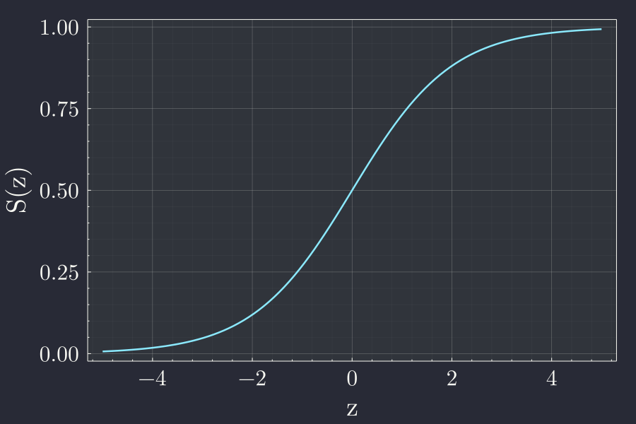
Lets define some activation function. A common activation function is the sigmoid function.

\[ \begin{aligned}S(z) = \frac{1}{1 + e^{-z}}\end{aligned} \]

S(z) = 1 ./ ( 1 .+ exp.(-z))

Since we also need the derivatives of activation function lets define that too.

\[ \begin{aligned}S^\prime(z) = \frac{e^{-z}}{\left(1 + e^{-z}\right)^2}\end{aligned} \]

S′(z) = exp.(-z) ./ ( 1 .+ exp.(z))

The sigmoid function looks like

x = range(-5,5,100);
y = S.(x)
plot(x,y)

I would like to write a very sparse function to implement the feedforward and back propagation.

function run(x,y;σ=S,σ′=S′)
    ŷ = y
    # Feed forward
    a⁰ = x
    z¹ = W¹ * a⁰ + b¹
    a¹ = σ(z¹)
    z² = W² * a¹ + b¹
    a² = σ(z²)

    # Calculate error
    δL = (a² - ŷ)
    # Back propagate error
    δ² = δL * σ′(z²)
    δ¹ = δ² * σ′(z¹) * W²
    # update biases
    global b² -= β * δ²
    global b¹ -= β * δ¹
    # update weights
    global W² -= β * δ²*a¹
    global W¹ -= β * δ¹*a⁰
    return a²
end

The code is exact one to one translation of mathematical expression we have defined. As explained in last post the weights and biases are updated in the direction opposite to the direction of gradient.

Lets generate some training samples

x_train = hcat(0:12...)
y_train = f.(x_train)

And train the network

epoch=1800
errs = []
for n in 1:epoch
    for (i,(x,y)) in enumerate(zip(x_train,y_train))
        ŷ = run(x,y)
        error = loss(y,ŷ)
        push!(errs,error)
        (n % 50 == 0) && print(f"\rEpoch {$n:>2d}: {$i:>02d}/{$(length(x_train)):>02d}   error = {$error:.3e}")
    end
    (n % 50 == 0) && println("")
end

Epoch 50: 16/16   error = 7.246e-03
Epoch 100: 16/16   error = 6.995e-03
Epoch 150: 16/16   error = 6.750e-03
Epoch 200: 16/16   error = 6.509e-03
Epoch 250: 16/16   error = 6.273e-03
⋮
Epoch 1650: 16/16   error = 1.587e-03
Epoch 1700: 16/16   error = 1.483e-03
Epoch 1750: 16/16   error = 1.383e-03
Epoch 1800: 16/16   error = 1.286e-03

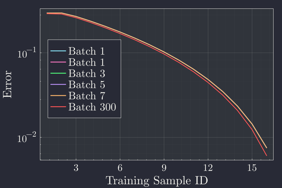
We see that the error goes down at the end of each epoch. Telling us that the back propagation works. But I can see that the error goes down much more slowly.

Conclusion

It is interesting to note that for the larger batch the error is not that improved from the early batches. I am guessing this is due to the fact that we are tyring to model a linear function with a non linear neural network. This tells us that our ability to train a particular dataset that might follow one functional form might not correctly be learned by a network that has other functional non linearlity.