Basic neural network with julia

In this post I will try to describe building a basic regression model with gradient descent. This forms a very basic prototype of neural network. This by no means is a full fledged neural network, but this makes very fundamental foundation of neural network. Feedforward to calculate the error and back propagation to update the weights and biases from the error function. The code cells can be collected into a script and run as an individual julia script to reproduce everything that is described here in this article.

Building a basic network

Lets say we want to fit a regression to some arbitrary linear expression. Lets assume such function be

f(x) = 5x + 3

Lets use a single perceptron neural network (?) to model this function. There will be a single perceptron connecting from input layer \(x\) to output layer \(f(x)\). Since there is a single perceptron, we will have 1 weight and 1 bias. Lets each initialize it to some random number.

W = rand(1);
b = [0];

#W = [0.19961796743719895] # #hide
W = [0.3890321538110373] #(upto -7) # hide

We can use weight and bias to predict the outcome. For a single perceptron neuron the prediction is simply \(Wx + b\) where \(W\) is the weight and \(b\) is the bias.

P(x) = W .* x .+ b

We can now choose a loss function, which can be an arbitrary metric that measures how far off from the true value is the prediction from network. Let such a error function be

This is simply a squared error function. The arbitrary scaling factor for the function doesn't matter much.

L(x,y)  = sum(y .- P(x)) .^ 2

The way our perceptron is going to work is we will have some set of known \(x\) and \(y\) that constitute to training set, which our network will use to learn about the actual regression parameters. Lets generate some numbers say \(\lbrace 0, 1 ,2 \cdots 5 \rbrace\). Since for our training set we have known values of output we will also calculate the true values of \(y\) for our training set.

x_train,x_test = hcat(0:15...), hcat(6:10...)
y_train, y_test = f.(x_train), f.(x_test)

With this we generated some data that we can use to train the network and later also test the network.

Lets see the loss function value at the without training the network, with the weights and biases randomly initialized.

x0,y0 = x_train[1], y_train[1]
initial_loss = L(x0,y0)
# returns 4.0

Our final output of the network is the function of input parameter along with weight and biases. For each learning step we want to change weights and biases such that the final output is closer to the desired output. We already have defined the loss function as a metric to measure this distance. Our parameters \(W\) and \(b\) have to change in a way that the metric gets closer if the parameter move close to the desired value. We can think of the ordered pair \((W,b)\) as a vector in a vector space and the loss function a scalar point function in this vector space. Our target is to find a vector in this space that minimizes the loss function.

This sounds awful lot like extremizing function in vector space. A fantastic mathematical tool that gives us the direction of change of metric with respect to change in some parameter of metric is the gradient aka derivative. We want to be calculating the gradient vector \((\nabla W,\nabla b)\) iteratively such that we get close to the target vector \((W_0, b_0)\).

The magic stuff from the neural network that actually allows it to "learn" is the gradient descent. The gradient in this vector space is

We then want to update our vector as

Lets use some arbitrary value for the learning rate \(\beta\). We will investigate the impact of this parameter later. For now lets just use

β = 0.05

For our simple network the gradient is fairly easy to calculate. Differentiating the loss function we get.

We can define these gradient function easily in julia.

∇W(x,y,W,b) = 2(y .- W .* x .-b ) .* ( .- x)
∇b(x,y,W,b) = 2(y .- W .* x .-b ) .* ( -1 )

Now that we have the gradient it is an easy task to just update the weight and bias vector.

gw = ∇W(x0,y0,W,b)
gb = ∇b(x0,y0,W,b)
W -= β * gw
b -= β * gb

If we calculate the loss function again at this point we should have made improvement in our weights and biases, so that the error should go down.

L(x0,y0)
# returns 3.24

The error indeed goes down. We can repeat this process of calculating the prediction with the training set, and updating the weights and biases with the gradient of loss function iteratively. Allowing us to converge the error to zero and the final weights and biases to the true weights and biases, which is also the coefficient of our target function.

epoch=5
for n in 1:epoch
    for (i,(x,y)) in enumerate(zip(x_train,y_train))
        W -= β * ∇W(x,y,W,b)
        b -= β * ∇b(x,y,W,b)
        error = loss(x,y)
        print("\rEpoch $n: $i/6   error = $(@sprintf("%.2e",error))")
    end
    println("")
end

println("Final equation : y = $(W)x+$b ")

Epoch 1:  6/6   Error = 1.144e+01
Epoch 2:  6/6   Error = 2.291e-01
Epoch 3:  6/6   Error = 4.970e-03
Epoch 4:  6/6   Error = 6.532e-05
Epoch 5:  6/6   Error = 7.673e-06
Final equation : y = 5.001279x  + 2.9991564

We see that at each epoch the error goes down and the final parameters is very close to the required initial parameters. As we can see the final parameters are very close to the actual value of the parameters we started with \(W=5\) and \(b= 3\).

The impact of learning rate

Now lets try to qualitatively see what happens with the change in learning rate. It is easy to modify above code to save the error value after each training sample for various learning rate. Apriori we do not know what learning rate to use. But a value close to \(1 \times 10^{-2}\) is a good starting point, that obviously depends upon the error function used. I ha For this exercise I will use the following list of learning rate.

βs = [0.09,0.08,0.07,0.06,0.051,0.04]

In the above exercise we calculated error after we updated the weights and bias after training with first sample \(x_0,y_0\), similarly we can do this for each \((x,y)\) is the batch of training set. In this example we are using the batch \(x_{train} = \lbrace 0,1,2,3,4,5 \rbrace\) and \(y_{train} = \lbrace 3, 8,13, 18, 23,28 \rbrace\)

Lets call \((x,y) = (0,3)\) and so on the samples. Since we repeated this process by feeding the same input again in the network for \(n=5\) (batchsize) times. For a single learning rate \(\beta\) we will have \(n=5\) curves of error corresponding to each batch. For \(\beta=0.09\) the error progression looks like

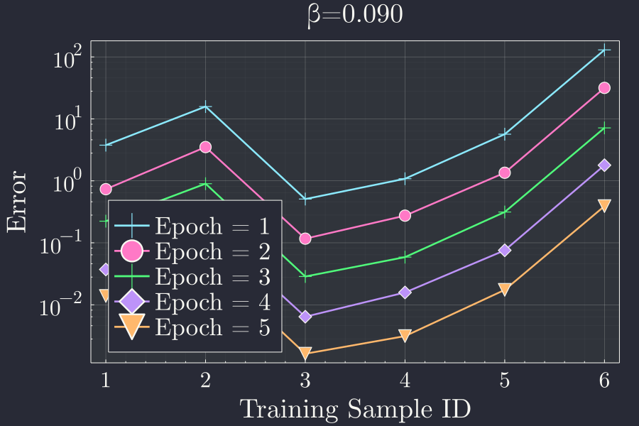
We see that the error progressively goes down each batch, but not necessarily across each training sample. This is expected because the initial random guess is very far off and the gradient is large causing more fluctuations. One important observation from this plot is that, even after training with fifth batch, the error is still high and the prediction is not close. This is because our choice of learning rate is not optimal.

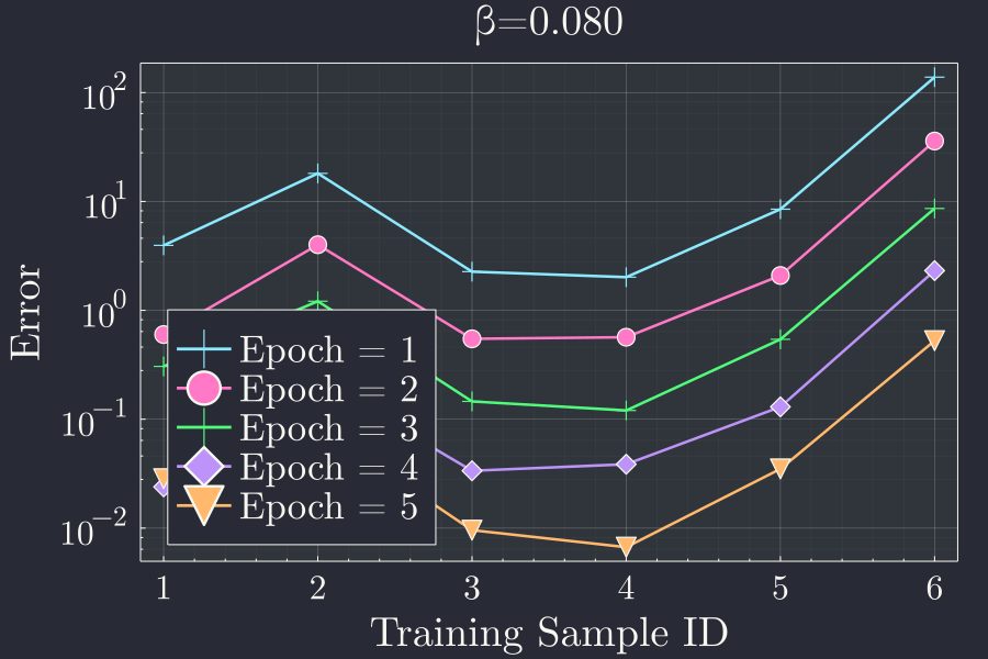
For a next learning rate \(\beta = 0.80\) the same plot looks like.

If we look at this plot for \(\beta = 0.051\) we get

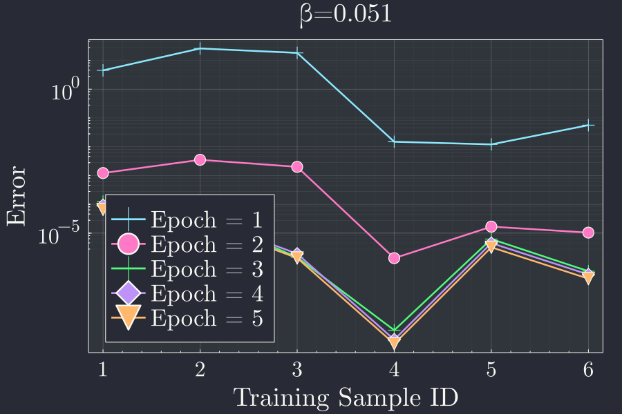
This is interesting to see that once we train our network with a optimal learning rate, the error quickly goes down each training sample after the first batch. In the first batch the network doesn't have.

As a summary we can plot the final error in each epoch vs the error in each epoch. This gives us an idea of how the error progresses for different learning rates in different epochs.

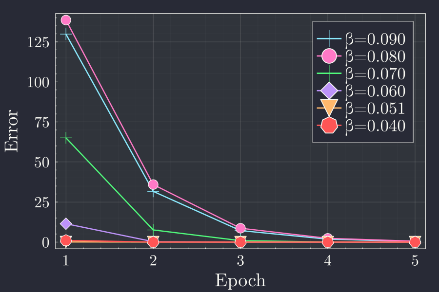
We see that with more epochs whatever the learning rate, the error goes down. This is to be expected because, more epoch to train means more time to adjust the weights and biases. To see the fluctation near the lower values of error we can see the same plot in logarithmic y axis.

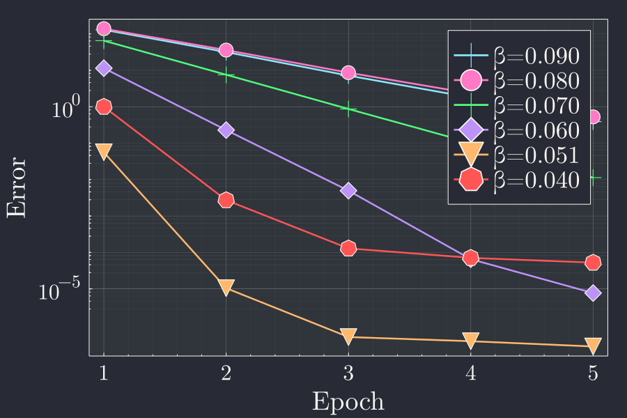
This gives a very clear idea of what training multiple epochs and for different learning rate does to the error of the prediction.

We can then plot the final error after the \(5^{th}\) epoch, for each learning rate \(\beta\) as a function of learning rate.

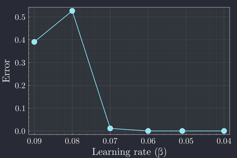
It seems that the learning rate smaller than \(0.070\) is good. A way to see the smaller variations in smaller values of the plot is to use logarithmic scale in the y axis to more closely see the variation.

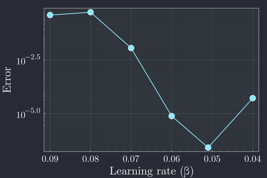
Here we see that after \(0.07\) any smaller learning rate gets the job done but importantly we also see that this is not a monotonic function. In fact the last point of the above plot has a slight bump, indicating going further down from \(0.05\) in fact causes the final error to be worse that the optimal value. This is the case of the network being overstrained. Instead of falling off to the optimal parameters it might wander off from it if we train it more than necessary. For this simple neural network, the even 6 training samples trained over 5 epochs is overtraining with learning rate of \(0.04\). We thus have to always be careful in selecting our sample size and the other hyperparameters like learning rate for the neural network. In the next post we will talk more about neural network with multiple neurons and possibly multiple hidden layer. Until then, hasta pronto.