Neutrino Mass Hierarchy

2024-07-28 · Prakash

Neutrinos

Neutrinos are little tiny particles that carry no charge and very little mass. The exact mass of neutrino is not known yet but, we know that they have very tiny mass. The confirmation of neutrino oscillation confirms that at least one neutrino is massive. In the current theory of neutrinos, we have three flavors of neutrinos corresponding to each charged lepton flavors.

What are lepton flavors? They are leptonic with similar characters and which participate similarly in the particle interaction, but have different masses depending on their nature. Although they are distinct particles, a massive similarity in their nature suggests a larger grouping into a single umbrella which we call the flavors.

Oscillation experiments allow us to calculate the (squared) difference of mass of neutrinos. Based on the data we have for the mass difference we can construct two possible mass ordering for the neutrinos. The mass of neutrinos also depend on the

Flavours of neutrino

When we detect neutrinos we detect the so called flavour eigenstates. In the 3 neutrino models theese are \(\nu_e\), \(\nu_\mu\) and \(\nu_\tau\). These three flavors of neutrinos are the ones that are observed. But these are not energy eignestates. The energy eigenstates are different. The transformation between these two different basis states is called the PMNS matrix

\[ \begin{aligned}\begin{pmatrix}U_{e1} & U_{e2} & U_{e3} \\ U_{\mu 1} & U_{\mu 2} & U_{\mu 3} \\ U_{\tau 1} & U_{\tau 2} & U_{\tau 3} \\\end{pmatrix}\end{aligned} \]

Using this matrix we can write the transformation as:

\[ \begin{aligned}\begin{pmatrix}\nu_e \\ \nu_\mu \\ \nu_\tau\end{pmatrix} = \begin{pmatrix} U_{e1} & U_{e2} & U_{e3} \\ U_{\mu 1} & U_{\mu 2} & U_{\mu 3} \\ U_{\tau 1} & U_{\tau 2} & U_{\tau 3} \\ \end{pmatrix} \cdot \begin{pmatrix} \nu_1 \\ \nu_2 \\ \nu_3 \end{pmatrix}\end{aligned} \]

The PMNS matrix is parameterized with angle parameters \(\theta_{13}\) and \(\theta_{23}\)

The \(0\nu\beta\beta\) is a rare second order process that will be one fo the keys to understanding the neutrino mass order.

Neutrino Sources

Majority of neutrinos produced on the sun are electron neutrionos \(\mu_\nu\) through a process of nuclear fusion in the sun's core. The process of formation of neutrinos on the solar core due to proton-proton reaction shown in the reaction below

\[ \begin{aligned}p + p = d + e^{+} + \nu_e\end{aligned} \]

The majority of solar neutrinos are produced by the reaction above. There are however other processes that also produce the neutrinos.

Another major source of neutrnios is the reactions in the earth's atmosphere. The atmospheric neutrinos are produced by the collison of cosmic rays mostly comrised of protons with the nuclei present in the upper atmosphere. This reaction produces a shower of hadrons most of which are pions. The pions then decay to a muon and muon neutrino. The muons further decay electron, muon and muon neutrino. Because of these series of reaction we can expect that the ratio of muon neutrino to electron neutrino in the atmospheric origin to be 2 to 1.

\[ \begin{aligned}\pi^+ & \to \mu^+ + \nu_\mu & \pi^- \to \mu^- + \bar{\nu}_\mu \\ \mu^+ & \to e^+ + \nu_e + \bar{\nu}_\mu & \mu^- \to e^- + \nu_e + \nu_\mu\end{aligned} \]

Althouth detailed calculations show other reactions and produce other neutrinos, these account for the most of atmospheric neutrinos.

Neutrino Oscillation

Since the mass eigenstates \(\nu_i\) and flavour eigenstates \(\nu_{e,\mu,\tau}\) are both orthogonal basis for 3-flavour neutrino basis states. Each can be expressed as linear combination of other basis states. As mentioned earlier this transformation from one basis to other is a Unitary 3 \(\times\) 3 matrix called the PMNS matrix. For example when a electron neutrino from solar reaction travels towards the earth, we can express at the origin, the solar neutrino (electron neutrino) eigenstate as linear combination of mass eigenstates

\[ \ket{\nu_e;0} = \sum_i U_{ei} \ket{\nu_i;0} P_{\nu_e \to \nu_\mu} \]

As the solar neutrino reaches the earth after finite time \(t\), we can express the eigenstate of same neutrino as

\[ \ket{\nu_e;t} \equiv \mathcal{U}(t) \ket{\nu_e; 0} = \sum_i U_{ei} \mathcal{U}(t)\ket{\nu_i;0} \]

The probability, then, of the same neutrino being detected as muon neutrino becomes

\[ \begin{aligned}P_{\nu_e \to \nu_\mu} = \left\lvert \left\langle \nu_\mu \vert \nu_e;t \right\rangle \right\rvert ^2 = \left\lvert \sum_i \bra{\nu_e} U_{ei}\mathcal{U}(t)\ket{\nu_i;0} \right\rvert ^2\end{aligned} \]

The time evolution operator \(\mathcal{U}(t)\) is a exponential function of Hamiltonian operator \(\mathcal{H}\) and so \(\ket{\nu_i}\) are eigenstates of the time evolution operator. The eigenvalues of the hamiltonian operator are.

\[ \langle{\mathcal{H}}\rangle = E_i = \sqrt{p_i^2 + m_i^2} \approx p_i + \frac{m_i^2}{2p_i} \]

Also for light neutrinos \(m_i \ll p_i \approx E\) where \(E\) is the total energy of particle.

Remembering the fact that the time evolution operator \(\mathcal{U}\) is exponential functionof hamiltonian \(\mathcal{H}\) we get

\[ \langle \mathcal{U} \rangle = e^{-i\left( E + \frac{m_i^2}{2E}\right) t} \]

Expressing \(\bra{\nu_\mu}\) as the linear combination of \(\bra{\nu_i}\) we get

\[ \begin{aligned}\bra{\nu_\mu} = \sum_i \bra{\nu_i} U^\dagger_{\mu i}\end{aligned} \]

Substuting back leads to a expression more or less like

\[ P_{\nu_e \to \nu_\mu} = \left\lvert \sum_i\sum_j \bra{\nu_j}U^\dagger_{\mu j} U_{ei}\mathcal{U}(t)\ket{\nu_i;0} \right\rvert^2 \]

Since \(\ket{\nu_i}\) are mutually orthogonal (because basis vectors), the above expression simplies to

\[ P_{\nu_e \to \nu_\mu} = \left\lvert \sum_i U^\dagger_{\mu i} U_{ei} e^{-i\left( E + \frac{m_i^2}{2E}\right) t} \right\rvert ^2 \]

Here \(E\) is constant so only acts as a phase factor for exponential function, so we can drop the phase factor when we calculate the absolute value. Also the time of travel is proportional to the distance of travel (\(L\)), combining all these lead to:

\[ P_{\nu_e \to \nu_\mu} = \left\lvert \sum_i U^\dagger_{\mu i} U_{ei} e^{-i \frac{m_i^2 L}{2E}} \right\rvert ^2 \]

I will go into the details of it in a different post but for now, we will take it as a fact that for two neutrino oscillation case, the equation simplifies to

\[ P_{\nu_e \to \nu_\mu} = \sin^2 (2\theta) \sin^2 \left( \frac{\Delta m^2 L}{4E}\right) \]

where \(\theta\) is such that \(\sin \theta = U_{e1}\) and \(\cos\theta = U_{e2}\) and \(\Delta m^2 \equiv \Delta m_{21}^2 = m_2^2 - m_1^2\). \(E\) as defined above is the starting energy of the originating neutrino and the is the distance between them.

Observation of Neutrino Oscillation

The measurement of neutrino oscillation gives us the LHS of the above equation. Using the known distance \(L\) and known energy \(E\) of the oscillating neutrino, with the use of \(\theta\) from experiments we can calculate the value of \(\Delta m^2\). So the oscillation experiments only give us the squared difference of mass of two neutrinos that oscillate.

In the real world, we can experimentally measure the squared mass difference of each pair of all three neutrinos mass eigenstate. Based on the difference of squared masses we can construct two different models.

If all that we know about neutrino masses is the squared difference, we cannot tell the absolute mass. But since we have constraints from mass difference.

Mass Hierarchy

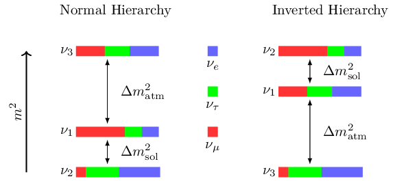
The different mass hierarchy possible with the measured experimental values are given names

Normal Hierarchy
Inverted Hierarchy

This figure shows the mass hierarchy

Finding the neutrino mass ordering is one of the unanswared questions of physics. One of the ways we can answer the question of mass ordering is by finding effective maojrana mass of the neutrinos. Which allows us to probe the possible region of neutrino masses. One very promising experiment that allows us to find the effective majorana mass is to measure the half life of neutrinoless double beta decay \(0\nu\beta\beta\) in certain nuclei. If we are able to precisely measure the half life of the \(0\nu\beta\beta\) process we can then infer the effective majorana mass, wich in turn will then allow us to figure out the neutrino mass hierarchy.

Neutrinoless double beta decay (\(0\nu\beta\beta\))

It is a rare second order process and we ca still type some \(\bra{\gamma}\) random stuffs.

Effective majorana mass

The effective majorana mass as a function of smallest neutrino mass is a topic of interest. The plot below shows the effective majorana mass as a function of lightest neutrino.

The mass data was taken from global fit

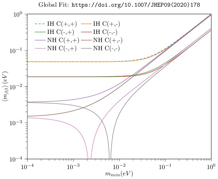
Figure 1. shows the possible curves for different CP violating parameters in the PMNS matrix elements.

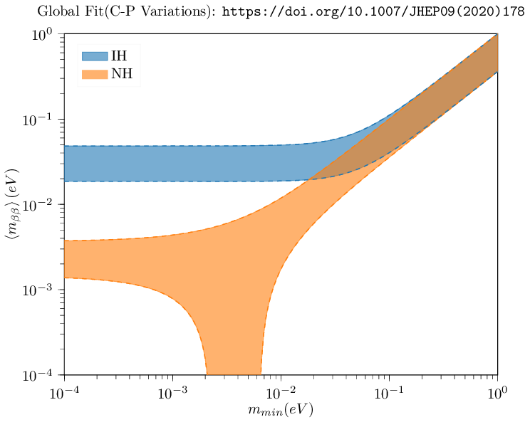
Figure 2. Shows the maximum uncertainity in Figure 1.

More will be written on this at a later time.