Discrete Fourier transform of Gaussian function

Introduction

This a a direct export from a jupyter notebook that I had for the study of discrete Fourier transfrom of Gaussian function.

import numpy as np
import sympy as smp
from sympy.utilities import lambdify
import matplotlib.pyplot as plt
plt.style.use(['dark_mode','slide_mode'])
import warnings
warnings.filterwarnings('ignore')

def vsplt(x1,y1,x2,y2):
    fig,ax = plt.subplots(1,2,figsize=(12,6))
    ax[0].plot(x1,y1)
    ax[1].plot(x2,y2)

def vstem(x1,y1,x2,y2):
    fig,ax = plt.subplots(1,2,figsize=(12,6))
    ax[0].stem(x1,y1)
    ax[1].stem(x2,y2)

mu,sigma = smp.symbols('mu,sigma',real=True,positive=True)
x = smp.symbols('x',real=True)
w = smp.symbols('omega',real=True)

I am trying to analyze the discrete fourier transform of gaussian function. I define a gaussian function first.

def Normal(x,mu,sigma):
    return 1/(sigma*smp.sqrt(2*smp.pi))*smp.exp(-smp.Rational(1,2)*((x-mu)/sigma)**2)

fnrm = Normal(x,mu,sigma); fnrm

\(\displaystyle \frac{\sqrt{2} e^{- \frac{\left(- \mu + x\right)^{2}}{2 \sigma^{2}}}}{2 \sqrt{\pi} \sigma}\)

I then calculate the fourier transform of the function (I could have made error in the factor in front though here)

ftr = smp.fourier_transform(fnrm,x,w); ftr

\(\displaystyle e^{2 \pi \omega \left(- i \mu - \pi \omega \sigma^{2}\right)}\)

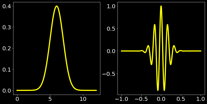
For continuous case I plot the gaussian function and its fourier transform. I choose the center of gaussian function cmu to be other than origin since it gives rise to interesting cases.

cmu = 6; csigma = 1
lfn = lambdify(x,Normal(x,cmu,csigma))
xrg = np.linspace(min(0,cmu-6),max(0,cmu+6),400)
xvl = lfn(xrg)
fptr = ftr.subs({mu:cmu,sigma:csigma}); fptr
lfptr = lambdify(w,fptr);

omg = np.linspace(-1,1,400)
fw = lfptr(omg)
vsplt(xrg,xvl,omg,fw); plt.show()

I take N samples taken in the range 0 and cmu+cmb because I am focusing only onn the right of imaginary axis now. From the analytic case above I already know what to expect for the fourier transform. But to my surprise the DISCRETE fourier transform of the sampled function is not what the analytic transform gave but half split and mirrored version of it.

N = 30; cmb = 15; N2 = int(N/2)
sample = np.linspace(0,cmu+cmb,N);
fsample = lfn(sample);
ftsample = np.fft.fft(fsample)
vstem(sample,fsample,range(len(ftsample)),ftsample)

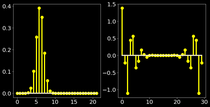
Apparant from the graph above on the right the fourier transform beyond N/2 should have appeared from -N/2 to 0 to match the analytic expectation. Next I do just that, I just lift off the part beyond N/2 and attach infront making it the exact sample of analytic expectation

#Now checking the inverse
iftsample = np.fft.ifft(ftsample)

#Reordering the samples in k space
nfsample = np.copy(ftsample);
nfsample[N2:] = ftsample[0:N2]; nfsample[0:N2] = ftsample[N2:]
#
fig,ax = plt.subplots(2,2,figsize=(14,12))
ax[0][0].stem(ftsample)
ax[0][1].stem(nfsample)
ax[1][0].stem(np.fft.ifft(ftsample))
ax[1][1].stem(np.fft.ifft(nfsample))
plt.show()

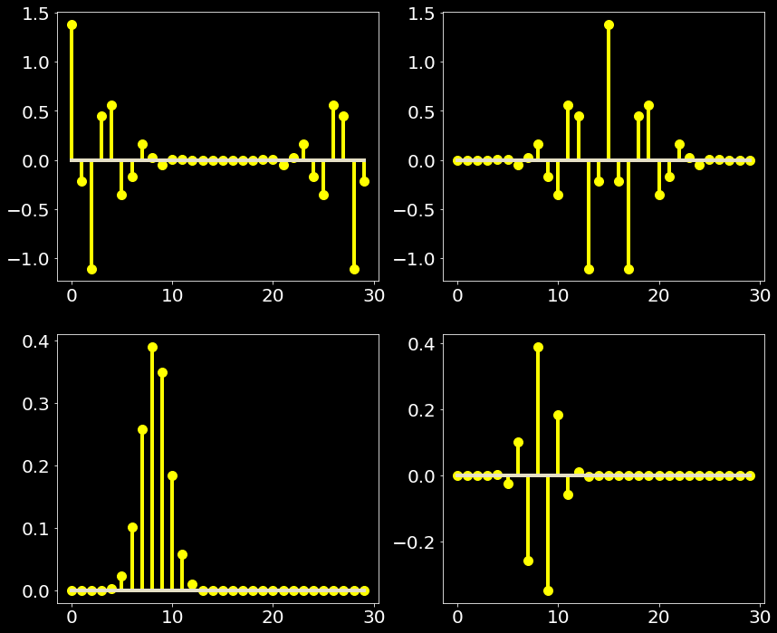
The top left graph of above plot is the DISCRETE fourier transform of the SAMPLE of function. The bottom left is the inverse DISCRETE fourier transform, the inverse transform gives back the signal. But the lifted-off-to-match-analytic-expectation samples do not transform exactly to the sample but now partially MIRRORED in real axis (meaning abs() of the inverse is the expected original sample).