Tikz

This is a figure I used for my homework at drexel . I drew it with very little knowledge of tikz at the time. %%A 2021-01-12 \usetikzlibrary{calc,patterns,angles,quotes} \begin{tikzpicture}[ thick, >=stealth, dot/.style = { draw, fill = white, circle, inner sep = 0pt, minimum size = 4pt } ] \coordinate (O) at (0,0); \coordinate (X) at (5,0); \coordinate (Y) at (0,4) ; \coordinate (A) at (-4,0); \coordinate (L) at (0,-1); \coordinate (U) at (0,4); \coordinate[label=above:P] (P) at (2,3); \coordinate (B) at (4,0) {}; \draw [dotted] (O) to node [below] {$d$} (A); \draw [dotted] (O) to node [below] {$d$} (B); \draw [-] (O) to node [below, sloped] {$r $} (P); \draw [dashed] (A) to node [sloped, above] {$r_2$} (P); \draw [dashed] (B) to node [sloped, above] {$r_1$} (P); % mirror \draw [-] (L) -- (U); \fill[black] (A) circle (0.13) node [circle,above,left, label=$-q$] {}; \fill [black] (B) circle(0.13) node [circle, above,right, label=$q$] {}; %\fill [gray] (O) circle(0.19) node [circle, above,left, label=$2q$] {}; \pic [draw, -, "$\theta$", angle eccentricity=1.5] {angle = B--O--P}; \end{tikzpicture}

\begin{tikzpicture} \node [anchor=west] (note) at (-1,3) {Curvature Note}; \node [anchor=west] (water) at (-1,1) {First Bump}; \begin{scope}[xshift=1.5cm] \node[anchor=south west,inner sep=0] (image) at (0,0) {\includegraphics[width=0.7\textwidth]{../tikz/complex_integration_2.png}}; \begin{scope}[x={(image.south east)},y={(image.north west)}] \draw[red,ultra thick,rounded corners] (0.48,0.80) rectangle (0.55,0.95); \draw [-latex, thick, red] (note) to[out=0, in=-120] (0.48,0.80); \draw [-stealth, line width=1pt, cyan] (water) -- ++(0.37,0.0); \end{scope} \end{scope} \end{tikzpicture}%

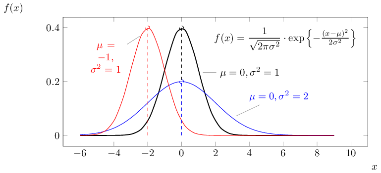
\begin{tikzpicture}[ declare function={ normalpdf(\x,\mu,\sigma)= (2*3.1415*\sigma^2)^(-0.5)*exp(-(\x-\mu)^2/(2*\sigma^2)); }, hplot/.style={ycomb, mark=o, dashed}] \begin{axis}[ width=12cm, height=6cm, samples=30, xlabel=$x$, ylabel=$f(x)$, xlabel style={at={(1,0)}, anchor=north west}, ylabel style={rotate=-90, at={(0,1)}, anchor=south east}, legend style={draw=none, fill=none}, domain=-6:9, legend cell align=left, xmin=-7, xmax=11] \addplot [smooth, thick] {normalpdf(x,0,1)} node[pos=0.47, pin={right:$\mu=0,\sigma^2=1$}] {}; \addplot [smooth, blue] {normalpdf(x,0,2)} node[pos=0.6, pin={45:$\mu=0,\sigma^2=2$}] {}; \addplot [smooth, red] {normalpdf(x,-2,1)} node[pos=0.25, pin={[text centered, text width=8ex] 200:$\mu=-1$, $\sigma^2=1$}] {}; \addplot [hplot, samples at={0}] {normalpdf(x,0,1)}; \addplot [hplot, samples at={0}, blue] {normalpdf(x,0,2)}; \addplot [hplot, samples at={-2}, red] {normalpdf(x,-2,1)}; \node[anchor=north east] at (axis description cs: 0.975, 0.95) {$f(x) = \dfrac{1}{\sqrt{2\pi\sigma^2}}\cdot \exp\left\{-\frac{(x-\mu)^2}{2\sigma^2}\right\}$}; \end{axis} \end{tikzpicture}

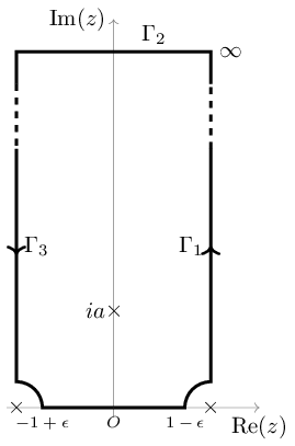
\begin{tikzpicture}[ contourline/.style={draw,line width=1.3pt} ] \tikzmath{\R=1.5;\r=0.4;\l=5;}% Change these values to see the magic \draw [help lines,->] (-\R*1.1,0) -- (\R*1.5,0) coordinate (xaxis); \draw [help lines,->] (0,-0.1*\R) -- (0,\l*1.2) coordinate (yaxis); \draw[contourline] (0,0) node [below, font=\scriptsize] (origin) {$O$} -- (\R-\r,0) node[below,font=\scriptsize]{$1-\epsilon$} arc(180:90:\r) node [below,font=\scriptsize]{} -- (\R,0.8*\l);% node [right] {$\infty$}; \draw[contourline] (\R,\l) -- (\R,1.1*\l)node [right] (infty) {$\infty$} -- (-\R,1.1*\l) --(-\R,\l); %\draw (\R,\l) -- (-\R,\l); \draw[dashed,contourline] (\R,0.8*\l) -- (\R,\l); \draw[dashed,contourline] (-\R,\l) -- (-\R,0.8*\l); \draw [contourline] (-\R,0.8*\l) node [below,font=\scriptsize] {} -- (-\R,\r) node [below,font=\scriptsize]{} arc(90:0:\r) node [below,font=\scriptsize]{$-1+\epsilon$} -- (0,0); \node at (-\R,0) {$\times$}; \node at (\R,0) {$\times$}; \node at (0,\l*.3) {$\times$}; \node [left] at (\R,0.5*\l) {$\Gamma_1$}; \draw [->,line width=1.1pt] (\R,0.5*\l); \node [above right] at (0.2*\R,1.1*\l) {$\Gamma_2$}; \node [right] at (-\R,0.5*\l) {$\Gamma_3$}; \draw [-<,line width=1.1pt] (-\R,0.5*\l); \node [left] at (0,\l*.3) {$ia$}; \node [below] at (xaxis) {Re($z$)}; \node [left] at (yaxis) {Im($z$)}; \end{tikzpicture}

\tikzset{ state/.style={ rectangle, rounded corners, draw=black, thick, minimum height=2em, minimum width=8em, inner sep=10pt, text centered } } \begin{tikzpicture}[>=latex, line width=0.75pt] \begin{scope} \node[state] (modelo1) {$x,y,z,r,\phi, x_{si},y_{si}$}; \node[below of=modelo1] {features}; \node (m1) [above right of=modelo1, node distance=3.5cm, matrix of math nodes, left delimiter=[,right delimiter={]}] { x_0 & y_0 & z_0 & r_0 & \phi& x_{s0}& y_{s0}\\ x_0 & y_0 & z_0 & r_0 & \phi& x_{s1}& y_{s1}\\ \vdots & \vdots & \vdots & \vdots & \vdots & \vdots & \vdots\\ x_n & y_n & z_n & r_n & \phi& x_{s0}& y_{s0}\\ x_n & y_n & z_n & r_n & \phi& x_{s1}& y_{s1}\\ \vdots & \vdots & \vdots & \vdots & \vdots & \vdots & \vdots\\ }; \node (m2) [right of=m1, node distance=4.5cm, matrix of math nodes, left delimiter=[,right delimiter={]}] { NOP_{\text{evtpos},\text{SiPMID}} \\ NOP_{\text{evtpos},\text{SiPMID}} \\ \vdots \\ NOP_{\text{evtpos},\text{SiPMID}} \\ NOP_{\text{evtpos},\text{SiPMID}} \\ \vdots \\ }; \node (modelo2) [right of=m2, state, node distance=3.7cm] (modelo2) {$NOP$}; \node[below of=modelo2] {output}; \path[->, shorten >=1em] (modelo1) edge[bend left=40] (m1.west); \path[->] (m1.south) edge[bend right=20] node [midway, below] {Model} (m2.south); \path[<-, shorten >=1em] (modelo2) edge[bend right=30] (m2); \end{scope} \end{tikzpicture}

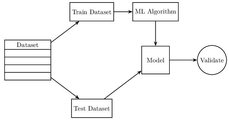
\usetikzlibrary{arrows.meta,shapes.multipart} \begin{tikzpicture}[ thick,>={Stealth[]}, ampersand replacement=\&, circ/.style = {draw,circle,minimum size=1cm}, rect/.style = {draw,rectangle,minimum size=1cm}, splt/.style = {draw,rectangle split,rectangle split parts=5,minimum size=0.5cm} ] \matrix[row sep=1cm,column sep=1cm] { {}; \& \node[rect] (Tr) {Train Dataset}; \& \node[rect] (A) {ML Algorithm}; \& {};\\ \node[splt, minimum size=25mm] (D) {Dataset}; \& {};\& \node[rect, minimum size=15mm] (M) {Model}; \& \node[circ] (V) {Validate};\\ {};\& \node[rect] (Te) {Test Dataset}; {}; \& {}; \&\\ }; \draw[->] (D) --(Tr); \draw[->] (D) --(Te); \draw[->] (Tr) --(A); \draw[->] (Te) --(M); \draw[->] (A) --(M); \draw[->] (M) --(V); \end{tikzpicture}

A sample diagram with custom defined function that also has legend. \begin{tikzpicture}[ declare function={ gamma(\z) = (2.50*sqrt(1/\z)+0.20*(1/\z)^(1.5)+ 0.00*(1/\z)^(2.5)-(174.21*(1/\z)^(3.5))/25920- (715.64*(1/\z)^(4.5))/1244160)*exp((-ln(1/\z)-1)*\z); }, declare function={ gammapdf(\x,\a,\b) = (\b^\a)*\x^(\a-1)*exp(-\b*\x)/gamma(\a); }] \begin{axis}[ width=9cm, height=6cm, samples=40, no marks, smooth, xlabel=$x$, ylabel=$f(x)$, xlabel style={at={(1,0)}, anchor=north west}, ylabel style={at={(0,1)}, anchor=south east}, legend style={draw=none, fill=none}, domain=0:22] \addplot[black] {gammapdf(x,3,1)}; \addlegendentry{$\alpha=3, \beta=1$} \addplot[blue] {gammapdf(x,8,1)}; \addlegendentry{$\alpha=8, \beta=1$} \addplot[red] {gammapdf(x,8,2)}; \addlegendentry{$\alpha=8, \beta=2$} \node[anchor=east] at (axis description cs: 1, 0.5) {$f(x) = \dfrac{\beta^{\alpha}}{\Gamma(\alpha)}\cdot x^{\alpha-1} \cdot \text{e}^{-\beta x}$}; \end{axis} \end{tikzpicture}

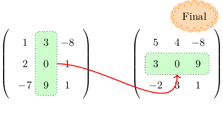
A helpful diagram to put in to annotate mathematical objects especially in beamer, where you can flip diagram and create a nice illustration. \begin{tikzpicture} \matrix (m) [matrix of math nodes, ampersand replacement=\&, left delimiter = (, right delimiter = ), nodes={minimum size=2em}] { 1 \& 3 \& -8\\ 2 \& 0 \& 1 \\ -7 \& 9 \& 1 \\ }; \matrix [matrix of math nodes, right =60pt of m-2-3.east, ampersand replacement=\&, left delimiter = (, right delimiter = ), nodes={minimum size=2em}] (j) { 5 \& 4 \& -8\\ 3 \& 0 \& 9 \\ -2 \& 3 \& 1 \\ }; \begin{pgfonlayer}{background} \draw[rounded corners, dotted, fill=green!20!white] (m-1-2.north west) rectangle (m-3-2.south east); \end{pgfonlayer} \begin{pgfonlayer}{background} \draw[rounded corners, dotted, fill=green!20!white] (j-2-1.north west) rectangle (j-2-3.south east); \end{pgfonlayer} \draw[->,thick,red] (m-2-2.east) to [out=0,in=270] (j-2-2.south); \node[draw=orange,cloud,double,fill=orange!30,cloud puffs=19, aspect=1.7,above right=1pt of j.north]{Final}; %\draw[cloud, above=30pt of m,fill=red,opacity=0.4] {Hello there}; \end{tikzpicture}

This diagram was made for my homework of Mathematical Physics at Drexel University during my Masters education The homework assignment can be found here at http://physics.drexel.edu/~pgautam/courses/ \begin{tikzpicture} [ %decoration={ % markings, % mark=at position 1cm with {\arrow[line width=1pt]{>}}, % mark=at position .3 with {\arrow[line width=1pt]{>}}, % mark=at position .6 with {\arrow[line width=1pt]{>}}, % mark=at position 0.8 with {\arrow[line width=1pt]{>}}, % mark=at position -5mm with {\arrow[line width=1pt]{>}}, %}, on each segment/.style={ decorate, decoration={ show path construction, moveto code={}, lineto code={ \path [#1] (\tikzinputsegmentfirst) -- (\tikzinputsegmentlast); }, curveto code={ \path [#1] (\tikzinputsegmentfirst) .. controls (\tikzinputsegmentsupporta) and (\tikzinputsegmentsupportb) .. (\tikzinputsegmentlast); }, closepath code={ \path [#1] (\tikzinputsegmentfirst) -- (\tikzinputsegmentlast); }, }, }, mid arrow/.style={ postaction={decorate, decoration={ markings, mark=at position .5 with {\arrow[#1]{stealth}} } } }, contourline/.style={line width=1.0pt}, axisline/.style={->,line width=0.3pt}, ] \tikzmath{\R=3;\r=0.5;\X=1.1*\R;\Y=1.1*\R;} \draw [axisline] (-\X,0) -- (\X,0) node [below right] {Re($z$)}; \draw [axisline] (0,1.2*\r) -- (0,-\Y) node[left] {Im($z$)}; \node at (0,0) {$\times$}; %\draw [contourline, postaction=decorate] \draw [contourline, postaction=={on each segment={mid arrow=red}}] (\r,0) node [below, font=\scriptsize] {$\epsilon$} -- (\R,0) node [above] {$R$} arc (0:-180:\R) node [above] {$-R$} -- (-\r,0) node [below, font=\scriptsize] {$-\epsilon$} arc (180:0:\r); \node at (\r,1.1*\r) {$\Gamma_{\varepsilon}$}; \node at (1.15*\R*0.7,-1.15*\R*0.7) {$\Gamma_{R}$}; % 0.7 = sin(45) = cos(45) \end{tikzpicture}

This diagram was made for my homework of Mathematical Physics at Drexel University during my Masters education The homework assignment can be found here at http://physics.drexel.edu/~pgautam/courses/ \begin{tikzpicture} [ decoration={ markings, mark=at position 0.10 with {\arrow[line width=1pt]{>}}, mark=at position 0.20 with {\arrow[line width=1pt]{>}}, mark=at position 0.30 with {\arrow[line width=1pt]{>}}, mark=at position 0.50 with {\arrow[line width=1pt]{>}}, mark=at position 0.70 with {\arrow[line width=1pt]{>}}, mark=at position 0.80 with {\arrow[line width=1pt]{>}}, mark=at position 0.90 with {\arrow[line width=1pt]{>}}, }, axes/.style={line width=0.1pt,->,opacity=.6, text opacity=1}, small/.style={font=\scriptsize} ] \tikzmath{\R=4;\r=0.7;}% Change these values to see the magic \draw [axes] (-\R*1.1,0) -- (\R*1.2,0) coordinate (xaxis) node [below] {Re$(z)$}; \draw [axes] (0,-0.1*\R) -- (0,\R*1.1) coordinate (yaxis) node [left] {Im$(z)$}; \node at (-0.5*\R,0) {$\times$}; \node at(-0.5*\R,0) [above] {$-\sigma$}; \node at (0.5*\R,0) {$\times$}; \node at (0.5*\R,0) [above] {$\sigma$}; \path [draw, line width=1.0pt, postaction=decorate] (0,0) -- (0.5*\R-\r,0) node [below,small]{$\sigma-\epsilon$} arc (180:0:\r) node [below,small]{$\sigma+\epsilon$} -- (\R,0) node [below] {$R$} arc (0:180:\R) node [below] {$-R$} -- (-0.5*\R-\r,0) node [below,small] {$-\sigma-\epsilon$} arc (180:0:\r) node [below,small] {$-\sigma + \epsilon$}-- cycle; \node at (0.5*\R,1.3*\r) {$\Gamma_{\varepsilon}$}; \node at (0.5*\R,0.8*\R) {$\Gamma_{R}$}; \end{tikzpicture}