Backpropagation

Setup

Similar to last post , where we made a basic neural network with just one neuron and no hidden layer, we will build a two neuron and a single hidden layer.

\begin{array}{r} a^{1} = W^{1} a^{0} + b^{1} \\ a^{2} = W^{2} a^{1} + b^{2} \end{array}

So the final output of the network as a function of $x$ input becomes

\begin{array}{r} y = W^{2} (W^{1} \cdot x + b^{1}) + b^{2} \end{array}

This is linear in $x$ . So we should be able to model any linear function with this network. Like before let us try to learn a linear model through this primite network. In the last post we trained the network to learn the linear model

\begin{array}{r} f (x) = 5 x + 3 \end{array}

Lets do the same with a new hidden layer as well. In julia we can declare the function

f(x) = 5x+3

\begin{array}{r} L (y, a^{2}) = {(y - a^{2})}^{2} \end{array}

Where $a^{2}$ is the true output and $y$ is the output from the network. Now again we want the loss function to minimize as we approach the correct model value for the model parameters. With the same approach we want to get the output.

The Algorithm (again)

\begin{array}{r} \frac{\partial L}{\partial W^{2}} = \frac{\partial}{\partial W^{2}} {(y - a^{2})}^{2} \\ = 2 (y - a^{2}) \frac{\partial a^{2}}{\partial W^{2}} \end{array}

\begin{array}{r} \frac{\partial a^{2}}{\partial W^{2}} = \frac{\partial (W^{2} a^{1} + b^{2})}{\partial W^{2}} = a^{1} \end{array}

\begin{array}{r} \frac{\partial L}{\partial W^{2}} = 2 (y - a^{2}) a^{1} \end{array}

\begin{array}{r} \frac{\partial L}{\partial W^{1}} = \frac{\partial}{\partial W^{1}} {(y - a^{2})}^{2} \\ = 2 (y - a^{2}) \frac{\partial a^{2}}{\partial W^{1}} \end{array}

\begin{array}{r} \frac{\partial a^{2}}{\partial W^{1}} = \frac{\partial (W^{2} a^{1} + b^{2})}{\partial W^{1}} = W^{2} \frac{\partial a^{1}}{\partial W^{1}} \end{array}

\begin{array}{r} \frac{\partial a^{1}}{\partial W^{1}} = a^{0} \end{array}

\begin{array}{r} \frac{\partial L}{\partial W^{1}} = 2 (y - a^{2}) W^{2} a^{0} \end{array}

\begin{aligned} \frac{\partial L}{\partial b^{2}} & = \frac{\partial}{\partial b^{2}} {(y - a^{2})}^{2} \\ = 2 (y - a^{2}) \frac{\partial a^{2}}{\partial b^{2}} \\ = 2 (y - a^{2}) \end{aligned}

\begin{aligned} \frac{\partial L}{\partial b^{1}} & = \frac{\partial}{\partial b^{1}} {(y - a^{2})}^{2} \\ = 2 (y - a^{2}) \frac{\partial a^{2}}{\partial b^{1}} \\ = 2 (y - a^{2}) W^{2} \end{aligned}

In all of the four derivatives above we see that the expression $(y - a^{2})$ appears. It might be worthwile to name that expression. Since it is the derivative and we are going to decrease the parameters $W^{2}, W^{1}, b^{2}, b^{1}$ proportional to this quantity, lets call it the error parameter and denote by $δ^{2}$ .

\begin{array}{r} (1) & δ^{2} = 2 (y - a^{2}) \end{array}

We also see that when we find the derivative of the loss function with the first set of paramters $W^{1}$ and $b^{1}$ , that the next weight $W^{2}$ is present. We can define

\begin{array}{r} (2) & δ^{1} = δ^{2} W^{2} \end{array}

Using these two definitions we cn write the four derivatives as.

\begin{aligned} \frac{\partial L}{\partial W^{2}} & = δ^{2} a^{1} \frac{\partial L}{\partial b^{2}} = δ^{2} \\ \frac{\partial L}{\partial W^{1}} & = δ^{1} a^{0} \frac{\partial L}{\partial b^{1}} = δ^{1} \end{aligned}

These are very symmetric equations from which we can immediately draw important conclusions.

We can think $δ^{2}$ in Eq. $(1)$ as the error in the last layer. Since these are used to update the weights and biases in the last layer. Particularly Eq. $(2)$ can be thought of as the error in the previous layer. The important conclusion is that the error in the previous layer $δ^{1}$ is proportional to the error in next layer $δ^{2}$ . So when we are applying this algorithm, we will first calculate the activation in each layers calculating $a^{n}$ s in each layer. This process is feeding the input forward in the network.

Once we have all the activations in each layer. We can first calculate the error in the last layer $δ^{2}$ and multiply with the weight in the last layer to calculate the error in previous layer $δ^{1}$ . We are essentially now propagating the error backwards in the network until we reach the first layer. Now it is very obvious why this process is called the backpropagation algorithm.

Implementation

Lets implement this algorithm in julia. First lets define the parameters

W¹, W², b¹,b² = 1.15,0.35, 0.0, 0.0

These are supposed to be random initial values to weights and biases. I have put constants here for the reproducibility of the result.

The loss function can be written as

L(y,a²) = (y-a²)^2

I would like to write a very sparse function to implement the feedforward and back propagation.

function train!(x,y)
    ŷ = y
    # Feed forward
    a⁰ = x
    a¹ = W¹*a⁰ + b¹
    a² = W²*a¹ + b²

    δ² = (a² - ŷ) # Calculate error
    δ¹ = (W² * δ²) # Back propagate error
    # update biases
    global b² -= β * δ²
    global b¹ -= β * δ¹
    # update weights
    global W² -= β * δ²*a¹
    global W¹ -= β * δ¹*a⁰
    return a²
end

The code is exact one to one translation of mathematical expression we have defined. As explained in last post the weights and biases are updated in the direction opposite to the direction of gradient.

Lets generate some training samples

x_train = hcat(0:12...)
y_train = f.(x_train)

And train the network

epoch=154
errs = []
for n in 1:epoch
    for (i,(x,y)) in enumerate(zip(x_train,y_train))
        ŷ = train!(x,y)
        error = loss(y,ŷ)
        push!(errs,error)
        print(f"\rEpoch {$n:>2d}: {$i:>02d}/{$(length(x_train)):>02d}   error = {$error:.3e}")
        #sleep(.15)
    end
    println("")
end

Epoch  1: 13/13   error = 4.776e+02
Epoch  2: 13/13   error = 4.755e-01
Epoch  3: 13/13   error = 5.525e-03
Epoch  4: 13/13   error = 7.767e-03
.
.
.
Epoch 152: 13/13   error = 1.280e-09
Epoch 153: 13/13   error = 1.170e-09
Epoch 154: 13/13   error = 1.068e-09

We see that the error goes down at the end of each epoch. Telling us that the back propagation works.

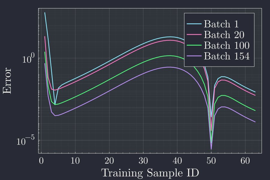
It is interesting to note that the error kind of adjusts itself to a shape after first batch and then after few batches settels on a shape. Then with more and more batches, the error converges towards zero. The particular shape of the error curve for different batches might be something worth investigating. But for now we will just take the final error all the samples in the batch is trained.

Conclusion

When we have multiple hiddne layer in the network, the final output is the composite function of all the functions till the last layer. So when we calculate the gradient of loss function with respect to the parameter in early layers of the network, it is not a easy job to calculate analytically, because the application of chain rule gets very complicated. But, with a slight change in approach, we can first calculate the erro in the last layer and express in the precedent layers just by using the weights as we would do in feeding input data to the ntework. This process of propagating the error in the final layer back to previous layers to find the errors in the previous layers is called the backpropagation algorithm.

To back propagate the error, we first feed the network and at each layer save the corrensponding weights biases and total activation. When we propagate the error back we use the same parameter that we saved earlier during feed forward. Thus with this clever idea a backpropagation we can calculate errors in the early layers of network by using the error in last layer propagated backwards.

Setup#

The Algorithm (again)#

Implementation#

Conclusion#

Setup

The Algorithm (again)

Implementation

Conclusion